
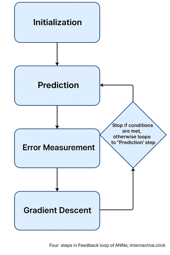
- Feedback loop when ANN learns
- TL;DR (90‑second summary)
- 1. Initialization – a rough first guess:
- 2. Prediction: Turning input into output:
- 3. Error Measurement – error as a difference between calculated and expected values:
- 4. Gradient Descent – update & Repeat:
- Building on the Basics – What Comes Next:
- All together how would the calculations work?
- Comparison to biological brain:
- Conclusion
- FAQs
- Sources and Further Reading:
Feedback loop when ANN learns
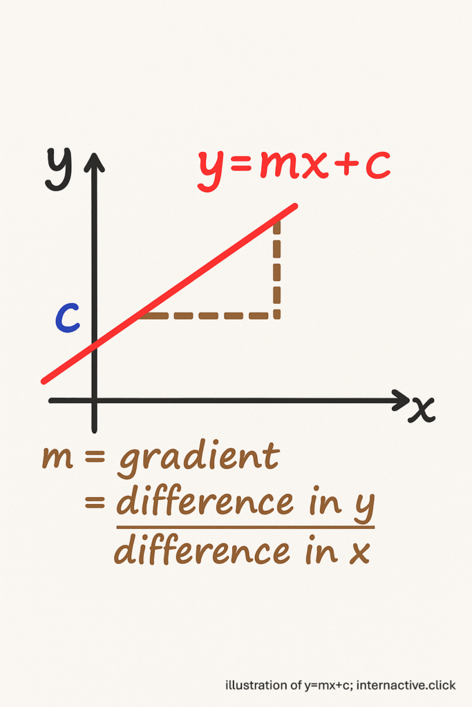
How exactly does an Artificial Neural Network Learn from Mistakes? We will use the straight line formula:
\( y = m x + c \)
which is one of the first equations most of us meet in middle school to explain. The core learning loop of an artificial neural network (ANN) is remarkably similar to fitting such a straight line to some data – only with many more “layers of equations” stacked together.
By revisiting this humble equation, we can watch the feedback loop – comparable to “nudging the shower knob until the water feels right” – the heartbeat of most ANN – unfold in four intuitive moves.
TL;DR (90‑second summary)
- Start with a guess. Initialise slope \(m\) and intercept \(c\) with small random values.
- Predict. For each input \(x\) compute \(y=mx+c\) (or \(y=max(0, mx+c)\) with ReLU in deep nets).
- Measure error. Compare predictions to true values using MSE
- Gradient Descent. Calculate gradients – that tells how much to tweak our initial values to get more accurate results
- Tweak & repeat. Use gradients to nudge \(m\) and \(c\) downhill until loss flattens.
This cycle powers everything from Amazon Alexa to self-driving cars.
Bonus deep dives: Feel free to ignore In-Depth, Optional Reading, and Q&A parts if you are here to just skim through the article.
1. Initialization – a rough first guess:
Analogy 1: When you turn on a radio: you start at static
Learning begins with uncertainty. The network assigns small random values to m (the slope) and c (the intercept).
Optional Reading: Why Random and Why Small Numbers
Why random? Because we are trying to find out the optimal values, we have to start somewhere. What’s more better than picking a direction in advance – to avoid favoring any particular direction. Imagine yourself covering your eyes and pointing at a map before beginning your treasure hunt.
Why small? Smaller numbers are easier to work with mathematically – trying \(5×3\) is more manageable than \(5,999,973×3\).
2. Prediction: Turning input into output:
Based on your current values, you calculate the predictions (\(\hat y\) pronounced y-hat).
For every training pair \((x,y)\) we plug \(x\) into our tentative line (in real nets, you’d also apply tiny hinge called ReLU, but we will skip that, check In-Depth 2) to get a predicted value
\( \hat y = mx +c \).
In a deep network this single algebraic step is replaced by many stacked layers, yet conceptually it’s the same: take the current parameters and produce output.
In-Depth: Understanding The Straight Line Formula
Toggle to Show/Hide
\(y\) vs \( \hat y\) -> \(y\) is the real output while \(\hat y\) is the predicted output.
This is where we flip the typical math class scenario. Normally your teacher gives you \(y = mx +c\) (with defined \(m\) and \(c\) values) and you plug in \(x\)’s. Here we flip the game: the data are fixed; the formula is what we’re hunting.
Remember the word problems where you solved for the equation of a line?
Consider this: If a line passes through \((0,1)\), \((1, 3)\), and \((2,5)\), you are working backwards to find the equation \(y = 2x + 1\). We start with a guess for \(m\) and \(c\) to calculate \(\hat y\).
In-Depth 2: Deeper Nets
Toggle to Show/Hide
In a true deep network, we would also calculate Rectified Linear Unit (ReLU), after each layer – check the attached figure:
\[z = Wx+b, then { a} = ReLU(z)\]
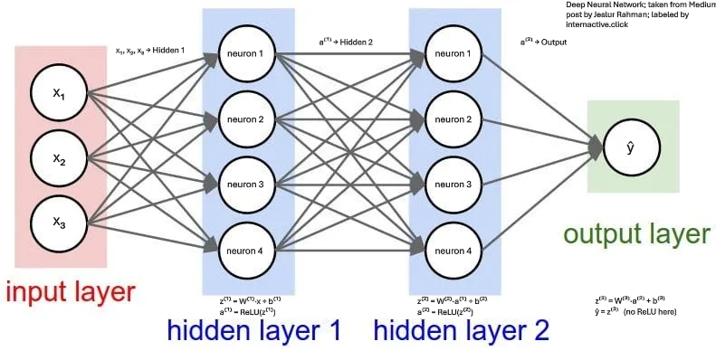
Each circle in Hidden 1 (and Hidden 2) represents a neuron with its own weight vector Wᵢ and bias bᵢ
From our simple demo, you can think of \(W\) and \(b\) as just \(m\) and \(c\). \(W\) is for weight and \(b\) is for bias. W is usually a set of weight values in a vector form as \(\{w1, w2, w3, w4\}\) and \(b\) as \(\{b1, b2, b3, b4\}\). Basically, the linear step \(y = mx + c\) gets wrapped in a gate that zeroes out negative values.
This concept echoes the biological All-or-Nothing principle, which describes how a neuron either fires a full action potential (if its input exceeds a threshold) or stays silent. If the signal is strong enough (positive), let it through; if not, don’t fire. \(ReLU\) (called an activation function) is inspired by it. If (\(mx+c\)) \(>0\), fire = \(mx+c\); else fire = 0.
In practice, you often let the very last layer remain linear (so the network can output any real number). All hidden layers (i.e., every layer except input and output) use ReLU (or another activation) to build up nonlinearity (in real life, many relationships- like friction, gravity, curves etc. – aren’t straight lines).
ReLU essentially asks “is this worth keeping?” for each calculation. By zeroing out negative values, it creates sparsity (lots of zeroes) which makes computations faster, and its mathematical simplicity (just taking the maximum among 0 versus the input) avoids certain training problems that plague other ReLU-like activation functions.
In-Depth 3: What are ReLUs?
Toggle to Show/Hide
Think of ReLU like an on/off switch:
- if the running value is positive, the switch lets it pass straight through.
- if it’s negative, the switch holds it at zero – like a one-way valve that blocks backward flow.
These little valves don’t matter for our single \(y=mx+c\) example, but once you stack many lines they let the combined curve bend, twist, and capture shapes a plain straight line never could.
3. Error Measurement – error as a difference between calculated and expected values:
The loss tells us the gap between prediction and reality.
Analogy 2: You sell a pen for $5, then notice everyone else charges $10. Loss = $10 - $5 = $5.
The most common choice for calculating this error is using Mean Squared Error (MSE):
\( MSE = \frac{1}{n}\sum_{i=1}^{n}\bigl(y_i – \hat y_i\bigr)^2\)
In plain English, take each true value y, subtract the prediction \( \hat y\), square the gap, add them all up, then divide by \(n\).
Optional Reading 2: How is MSE or Loss Calculated
1. Let’s say we have three data points: \[ (x_1,y_1) = (0, 1), (x_2, y_2)=(1,3), (x_3, y_3)=(2,5)\]. So \(n =3\).
2. Suppose our randomly assigned values for the line is: \[\hat y = mx+c\]
with \(m =2, c=5\)
Then for each \(x_i\) we calculate the predicted value \(\hat y_i\):
\[\hat y_1 = 2×0 + 5 = 5, \hat y_2 = 2×1 +5=7, \hat y_3 = 2×2+5=9\]
3. Now, the “error” or “residual” at each point is \(\hat y_i – y_i\). In our case:
\[y_1-\hat y_1 = 1-5 =- 4, y_2-\hat y_2 = 3-7=-4, y_3-\hat y_3 = 5-9 = -4\]
4. To get MSE, we square each residual and average over all \(n=3\) points:
\[ MSE = \frac{1}{n}\sum_{i=1}^{3}\bigl(y_i – \hat y_i\bigr)^2 = (-4)^2+(-4)^2+(-4)^2 = 16+16+16 = 48\]
\[MSE = \frac{1}{n}\sum_{i=1}^{n}\bigl(y_i-\hat y_I\bigr)^2 = \frac{48}{3} = 16\]
Therefore, the MSE at this step is 16. You would then use that value (or its gradient) to update \(m\) and \(c\) in the next iteration of your feedback loop.
4. Gradient Descent – update & Repeat:
Compute gradients – which tells us how steep the error hill is at a point – with respect to \(m\) and \(c\), and update them to minimize error:
\(m_{\text{new}} = m_{\text{old}} – \alpha \frac {\partial \operatorname {MSE}}{\partial m} \)
and \(c_{\text{new}} = c_{\text{old}} – \alpha \frac{\partial \operatorname{MSE}}{\partial c}\)
where \(\alpha\) (pronounced alpha) is the learning rate – higher the rate, the bigger the change in values of \(c\) and \(m\) every time we go through this feedback loop.
In those two equations, we move each parameter a small step in the direction that reduces the loss (the slope of the loss function at our current \(m\) and \(c\).
Analogy 1 contd.: Twist the radio knob slightly towards clearer music; too big a twist and you overshoot the station
Analogy 2 contd.: To reduce your loss of $5, you raise by $5 -> $10. Same idea - adjust the direction that shrinks the loss.
Finally, we circle back to Step 2 with the new \(m\) and \(c\), measure the new error, compute fresh gradients, and tweak again. We keep looping – guess -> predict -> measure -> tweak – until the error stops shrinking or we complete a set number of epochs (repetitions).
Note that because we base our demo on a single line, we compute the gradients by hand. In a real multi-layer network, the same “tweak” step is done automatically by back-propagation, which applies the chain rule (a concept from calculus) to send the error signal backward through each layer.
Now that you understand the core learning loop, let’s explore how this simple concept scales up to create the powerful AI systems you hear about in the news. Each of the following concepts builds directly on our straight-line example.
Building on the Basics – What Comes Next:
- From one line to a multilayer stack:
A single line only tilts; stack many lines with ReLU gates and the pieces bend into any curve.
Picture Lego bricks clicking together so a flat tile grows into a sculpted arch.
For maths enthusiasts, you must have heard the argument that a circle is made of a combination of straight lines – represented by tangent – if you draw a small line followed by subsequent lines that tilt further slightly in the same direction, you will end up with a circle. - Back-prop mechanics:
In a multilayer neural network, the “tweak” step from our feedback loop involves a back-propagation algorithm that quietly works out how much each connection caused the mistake and nudges all of them.
Think of it like rewinding your TikTok dance to the exact step where you tripped, then fine-tuning every move so the whole routine lands smoothly. - Practical Training Hygiene
Train on mini-batches (small, shuffled groups of examples) so each update is quick and focused; use a separate validation set as your honest “pop quiz” to catch overfitting (when the model memorizes training data but fails on new examples); and employ early-stopping so you halt training the moment that validation score ceases to improve.
Imagine learning a new language with flashcards: you study shuffled decks of words in small batches, quiz yourself on unseen cards to check real progress, and stop drilling once you’re acing every pop quiz. - Vectorization and Matrix form:
Replace our simple m and c with massive matrices W and vectors x (mathematical structures that organize thousands of numbers) so GPUs can crunch thousands of parameters simultaneously instead of one at a time. This is where NVIDIA and similar GPU powerhouses shine – they devour vectorized matrix calculations like popcorn.
It’s like hiring a moving truck to haul every box at once instead of carrying them down the stairs one by one. - Regularization techniques:
Weight decay and dropout act as gentle brakes that prevent the model from memorizing random noise in your training data, forcing it to learn genuine patterns instead.
Prune a bonsai tree so only the strongest, most essential branches remain – the result is more elegant and resilient. - Beyond MSE – Different scorecards for different games:
Swap Mean Squared Error for cross-entropy when predicting categories, accuracy for simple classification tasks, or ROC-AUC when you care about ranking. Each problem type deserves its own measuring stick.
Different sports need different scoreboards – you wouldn’t judge a basketball game by golf rules.
All together how would the calculations work?
- Initialize the Parameters:
Let’s start with initial guesses \(m = 2\), \(c = 5\), for data points \(x,y\) = \(\{(0,1), (1,3), (2,5)\} \). - Calculate Predictions and MSE
Predicted outputs using our initial guess are:
\[ \hat y = mx+c = \{2×0+5, 2×1+5, 2×2+5\} = \{5, 7, 9\}\]
Now, Mean Squared Error(MSE):
\[ MSE_{\text {old}} = \frac{1}{n}\sum_{i=1}^{n}\bigl(y_i-\hat y_i\bigr)^2 = \frac{(1-5)^2+(3-7)^2+(5-9)^2}{3} = \frac{16+16+16}{3} = 16 \] - Compute Gradients
Gradients tell us how to tweak parameters to reduce error.
Gradient w.r.t. slope (m):
\[ \frac {\partial \operatorname{MSE}}{\partial m} = -\frac{2}{n} \sum_{i=1}^{n}\bigl(y_i-\hat y_i\bigr)x_i \]
Calculating explicitly:
– Differences: \( (y – \hat y) = \{ -4, -4, -4\} \)
– Multiplying by \(x\): \( (-4)*0+(-4)*1+(-4)*2 = – 12\)
– Hence, gradient: \[ \frac{\partial \operatorname {MSE}}{\partial m} = \frac {2}{3}(-12) = 8 \]
Gradient w.r.t. intercept (c): \[ \frac{\partial \operatorname{MSE}}{\partial c} = – \frac {2}{n}\sum_{i=1}^{n}\bigl(y_i – \hat y_i\bigr) = \frac {-2}{3}(-12) = 8 \] - Update Parameters (Gradient Descent step):
Choose learning rate (\(\alpha\)) = \( 0.1\):
– Slope update: \[\Delta m = -\alpha \frac{\partial \operatorname{MSE}}{\partial m} = -0.1*8 = -0.8 \]
Thus, \[m_{\text{new}} = m_{\text{old}} + \Delta m = 2-0.8 = 1.2 \]
– Intercept update: \[\Delta c = -\alpha \frac{\partial \operatorname{MSE}}{\partial c} = -0.1*8 = -0.8 \]
Thus, \[c_{\text{new}} = c_{\text{old}} + \Delta c = 5-0.8 = 4.2 \] - Optional: Recalculate the MSE with new parameters:
With \(m = 1.2\) and \(c=4.2\):
– New predictions: \[\hat y_{\text{new}} = \{4.2, 5.4, 6.6\}\]
– New MSE: \[MSE_{\text{new}} = \frac{(1-4.2)^2+(3-5.4)^2+(5-6.6)^2}{3}\] = \frac{10.24+5.76+2.56}{3} = 6.19\]
Thus, we clearly reduced the error: \[ Loss_{\text{change}} = MSE_{\text{new}} – MSE_{\text{old}} = 6.19-16 = -9.81\] - Rinse and Repeat:
Now, repeat this process (predict, measure error, calculate gradients, update parameters) – steps 2-5 – until the loss no longer significantly decreases or until a predefined epoch limit is reached.
Comparison to biological brain:
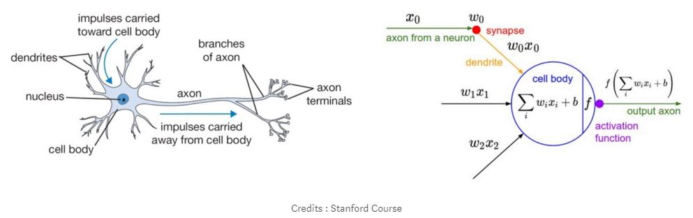
While biological brains work very differently from artificial networks, they do share some conceptual similarities in how they adapt and learn:
– Signal propagation LIKE prediction – An input spike travels through axons and synapses to create an output spike – analogous to y-hat.
– Error signals LIKE loss gradients – Neuromodulators like dopamine broadcast “better-than-expected” or “worse-than-expected” outcomes, telling distant synapses whether to strengthen or weaken.
– Synaptic plasticity LIKE parameter update – Hebbian rules (“cells that fire together wire together”) and their modern cousins adjust weights, nudging the circuit toward more accurate future responses.
In-Depth 4: How engineers borrow brain tricks
Toggle to Show/Hide
Brains don’t sit around doing calculus. They fine-tune themselves through tiny chemical nudges, not by cranking out partial derivatives. Neural networks copy that idea, not the exact biology: they keep adjusting their digital “connections” whenever feedback says the answer is off. You can spot the homage all over modern AI—Convolutional Neural Network (CNN): edge-finding filters that echo the visual cortex, transformers (think about the T in GPT): attention layers that shift focus like your own gaze, and Reinforcement-Learning Agents: game-playing agents that chase a digital “dopamine” reward signal.
| AI building block | What it does in plain English | Brain hint | Everyday analogy |
| Convolution (CNN) | Slides a small window across a picture to spot edges and blobs. | Early visual cortex cells fire for tiny oriented bars. | Like dragging a stencil over a photo to highlight outlines. |
| Attention (Transformers) | Lets the model zoom in on the most relevant words or pixels each step. | The brain’s spotlight of attention boosts wanted signals, dims noise. | You tune out chatter at a party to hear your name. |
| Reinforcement learning | Gives the agent a single score (reward) after each action; it learns to score higher next time. | Dopamine bursts = “better than expected”, dips = “worse”. | Getting more coins in a video game tells you which moves to repeat. |
It’s important to note that these are conceptual parallels, not exact equivalents. Real brains use complex biochemical processes that we’re still discovering, while artificial networks use precise mathematical calculations. AI researchers borrow the general principles rather than copying biology directly.
Conclusion
In a nutshell, training a neural network is just a loop of four steps – “guess -> predict -> measure -> tweak” – using ideas from the simple line \(y = mx+c\). We start with random \(m\) and \(c\), predict \(\hat y\), calculate how far off we are (MSE), then adjust \(m\) and \(c\) by a small amount (gradient descent). Stack many of those “linear step + ReLU gate” layers, and the network can bend straight lines into complex curves. Whether you’re fitting one line or a huge transformer model, the same basic loop applies – just on a bigger scale.
FAQs
Q: Does this provide a complete picture?
A: Not really, just the tip. However, it goes through all of the basic functionalities of ANN. The article attempts to summarize and hopefully create a rough prototype visualization of what ANN or Artificial Neural Network in the AI space are. You can advance up from here.
Q: Do real brains calculate derivatives?
A: No—biological neurons adjust via local signals and synaptic plasticity, but the backpropagation algorithm is inspired by gradient ideas rather than literal biology.
Q: Why use ReLU instead of linear?
A: ReLU introduces non‑linearity so networks can bend to fit curves rather than straight lines only. It’s like cutting off negative values to allow sharper model responses.
Q: What if my model stalls before fitting well?
A: You may need to adjust the learning rate, add momentum, or re‑initialize parameters.
Sources and Further Reading:
- Foundational Texts on Deep Learning
- Goodfellow, I., Bengio, Y., & Courville, A. (2016). Deep Learning. MIT Press.
- Excellent for understanding backpropagation, activation functions, and the mathematics behind gradient-based learning.
- Nielsen, M. (2015). Neural Networks and Deep Learning. (Available at http://neuralnetworksanddeeplearning.com/)
- A very accessible, hands-on walk-through of feedforward networks, gradient descent, and the intuition behind each step.
- Goodfellow, I., Bengio, Y., & Courville, A. (2016). Deep Learning. MIT Press.
- Activation Functions & ReLU
- Ramachandran, P., Zoph, B., & Le, Q. V. (2017). “Searching for Activation Functions.” arXiv:1710.05941.
- Covers various activations (including ReLU variants), empirical comparisons, and why ReLU became so popular in practice.
- Ramachandran, P., Zoph, B., & Le, Q. V. (2017). “Searching for Activation Functions.” arXiv:1710.05941.
- Online Courses (including Andrew Ng’s deeplearning.ai)
- Ng, A. (2023). Deep Learning Specialization. deeplearning.ai (https://www.deeplearning.ai/).
- A step-by-step series of courses covering neural networks, backpropagation, and modern practices (with code examples in Python/TensorFlow).
- Especially useful if you want guided exercises on implementing ReLU layers, loss functions, and gradient descent from scratch.
- Coursera: Ng, A. (2023). “Neural Networks and Deep Learning” (Course 1 of the Deep Learning Specialization).
- Focuses on core concepts—initialization, forward propagation, ReLU/nonlinearities, and backprop—for a solid practical foundation.
- Ng, A. (2023). Deep Learning Specialization. deeplearning.ai (https://www.deeplearning.ai/).
- Neuroscience & Biological Inspiration
- Lillicrap, T. P., Santoro, A., Marris, L., Akerman, C. J., & Hinton, G. (2020). “Backpropagation and the Brain.” Nature Reviews Neuroscience, 21(6), 335–346. https://doi.org/10.1038/s41583-020-0277-3
- Explains which aspects of gradient-based learning mirror biological synaptic plasticity, and which are purely engineered.
- Hochreiter, S., & Schmidhuber, J. (1997). “Long Short-Term Memory.” Neural Computation, 9(8), 1735–1780.
- Not directly about ReLU, but a classic when you later explore how gating ideas in RNNs borrow loosely from biology.
- Lillicrap, T. P., Santoro, A., Marris, L., Akerman, C. J., & Hinton, G. (2020). “Backpropagation and the Brain.” Nature Reviews Neuroscience, 21(6), 335–346. https://doi.org/10.1038/s41583-020-0277-3
- Loss Functions & Optimization
- Bishop, C. M. (2006). Pattern Recognition and Machine Learning. Springer.
- Chapters on error functions (MSE, cross-entropy), gradient descent variants, and regularization techniques.
- Bishop, C. M. (2006). Pattern Recognition and Machine Learning. Springer.
- Practical Tutorials and Code Examples
- Chollet, F. (2017). Deep Learning with Python (Manning).
- Hands-on Keras/TensorFlow examples that let you see exactly how ReLU, MSE, and gradient descent are implemented.
- Stanford CS231n: Convolutional Neural Networks for Visual Recognition (Lecture notes, 2023).
- Provides clear notes on ReLU, forward/backward passes, and common pitfalls—good companion reading if you want deeper intuition.
- Chollet, F. (2017). Deep Learning with Python (Manning).
This article synthesizes foundational principles from authoritative textbooks and peer-reviewed articles in deep learning and neuroscience. Sources have been selected to balance accuracy, clarity, scientific rigor, and reflect consensus view within AI research communities.